Validation

liulu is validated against \(N\)-body halo catalogues (LCDM and \(f(R)\) fiducial cosmologies, \(z=0.25\), up to 100 boxes, four mass cuts). The full study is in the companion LaTeX report (docs/streaming_model_report.tex); this page summarises the conclusions and key figures.

The model is correct and literature-consistent

Feeding measured \(\xi(r)\) and pairwise velocity moments through the streaming integral reproduces the measured redshift-space multipoles at the expected accuracy: \(\xi_0\) to sub-percent (at \(s>3\,\mathrm{Mpc}/h\), with the log–log \(\xi(r)\) default) and the skew-\(t\) \(\xi_2\) to a few percent on quasi-linear scales.

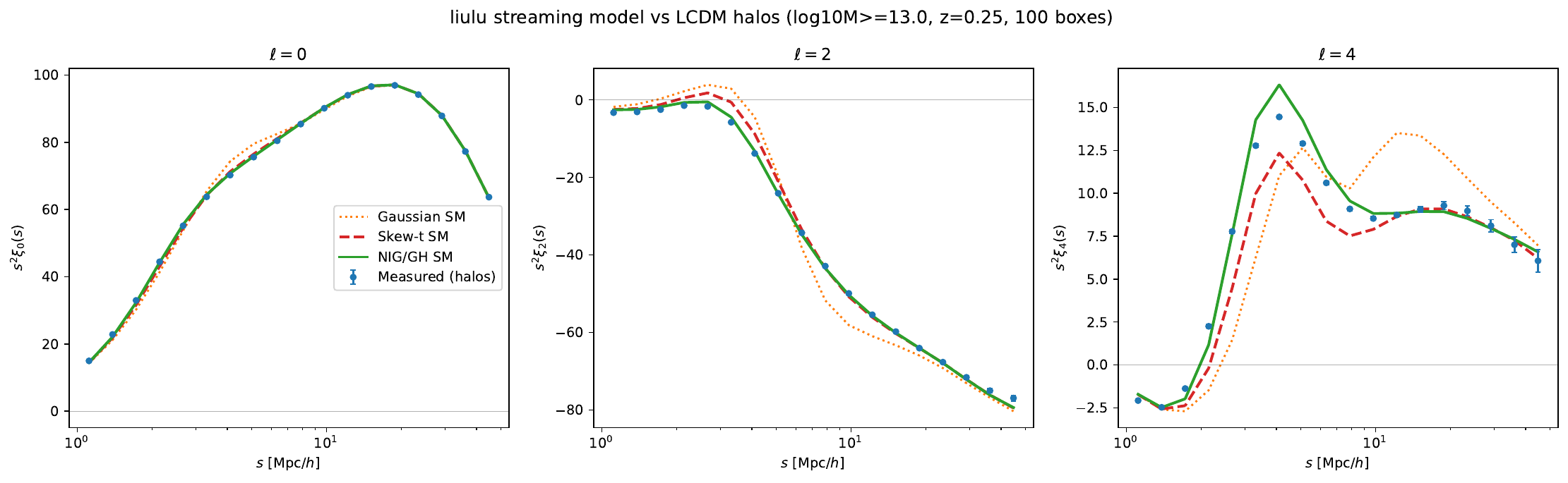
The quadrupole-dip problem and its fix

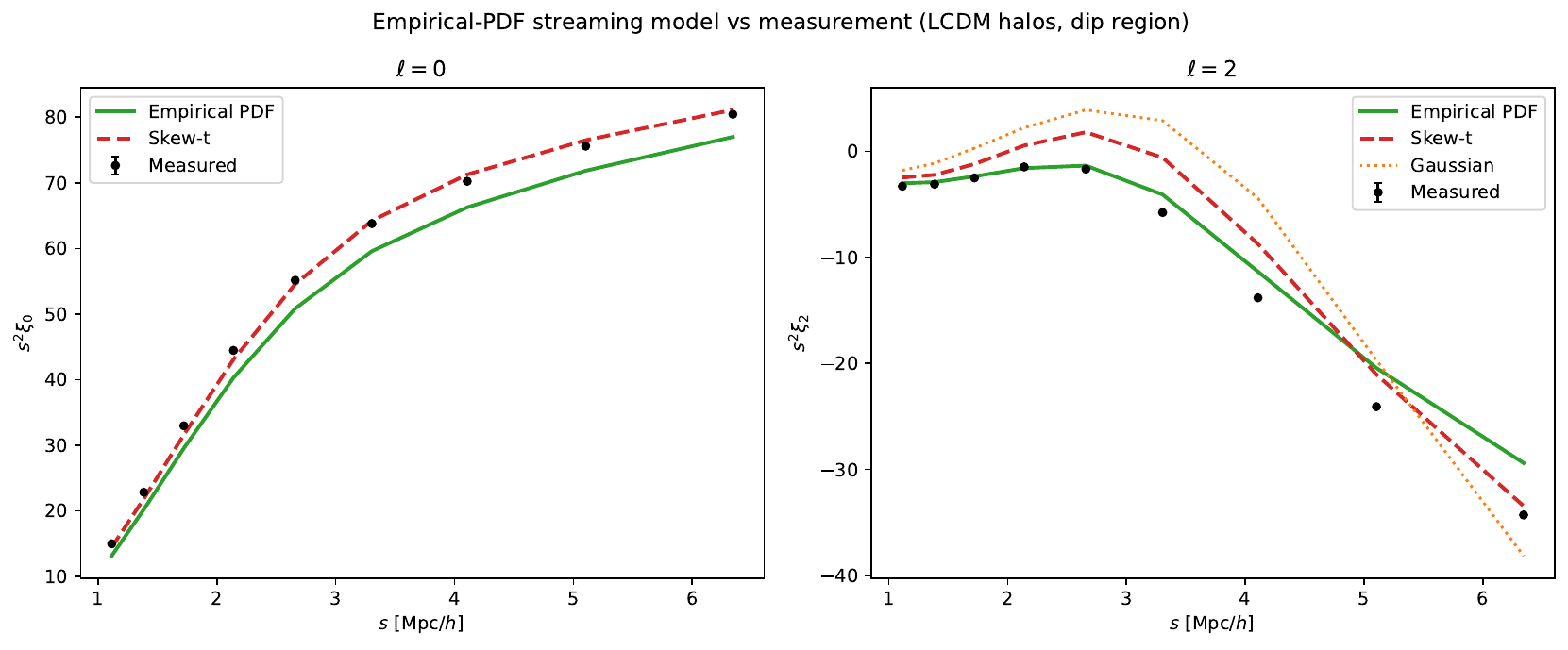
The residual in \(s^2\xi_2\) around \(s\sim3\)–\(5\,\mathrm{Mpc}/h\) — the Fingers-of-God → Kaiser transition — is not numerical: it is the intrinsic limitation of the four-moment skew-\(t\) shape. The distinct-halo pairwise velocity PDF there is skewed and leptokurtic (from the intrinsic non-Gaussianity of the velocity field plus an environmental superposition over pairs; there is no 1-halo term for distinct haloes).

Feeding the empirically measured velocity PDF through the exact integral roughly halves the residual, confirming the gap is the PDF shape, recoverable with a better PDF model:

NIG fixes most of it

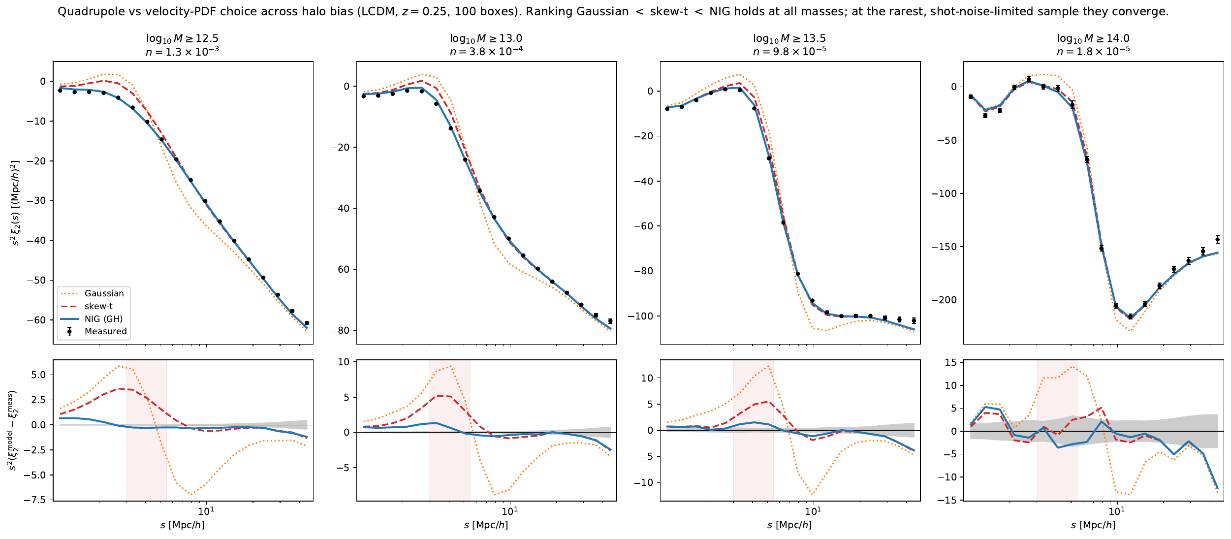
Replacing the skew-\(t\) with the NIG (generalized-hyperbolic) PDF — same four moments, a Gaussian-mixture shape — cuts the \(\xi_2\)-dip residual from ~35% to ~3%, while keeping the monopole at ~1%. The improvement is robust across tracer bias (four mass cuts) and to modified gravity (\(f(R)\)): NIG improves the \(\xi_2\) \(\chi^2/\mathrm{ndof}\) over the skew-\(t\) by ~10–25× for well-populated samples.

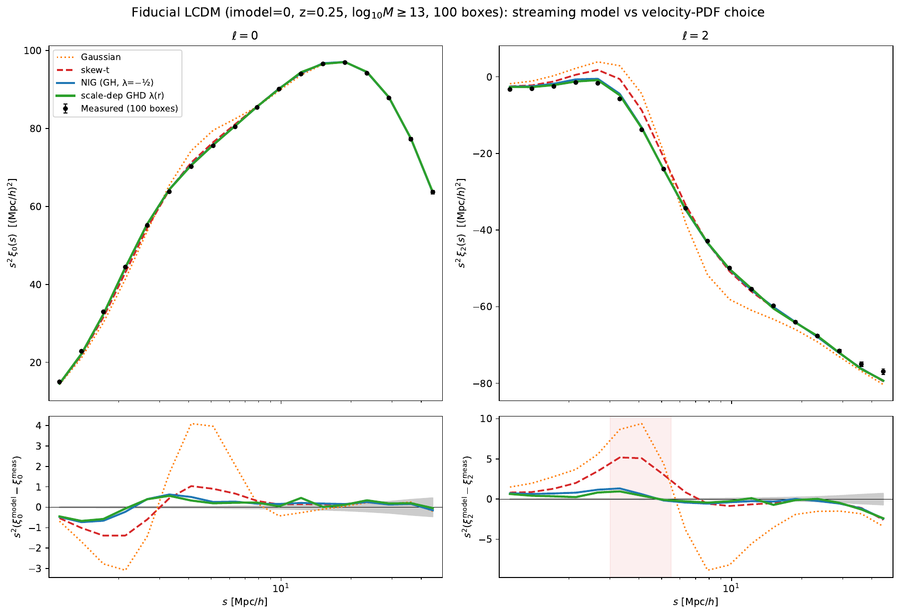
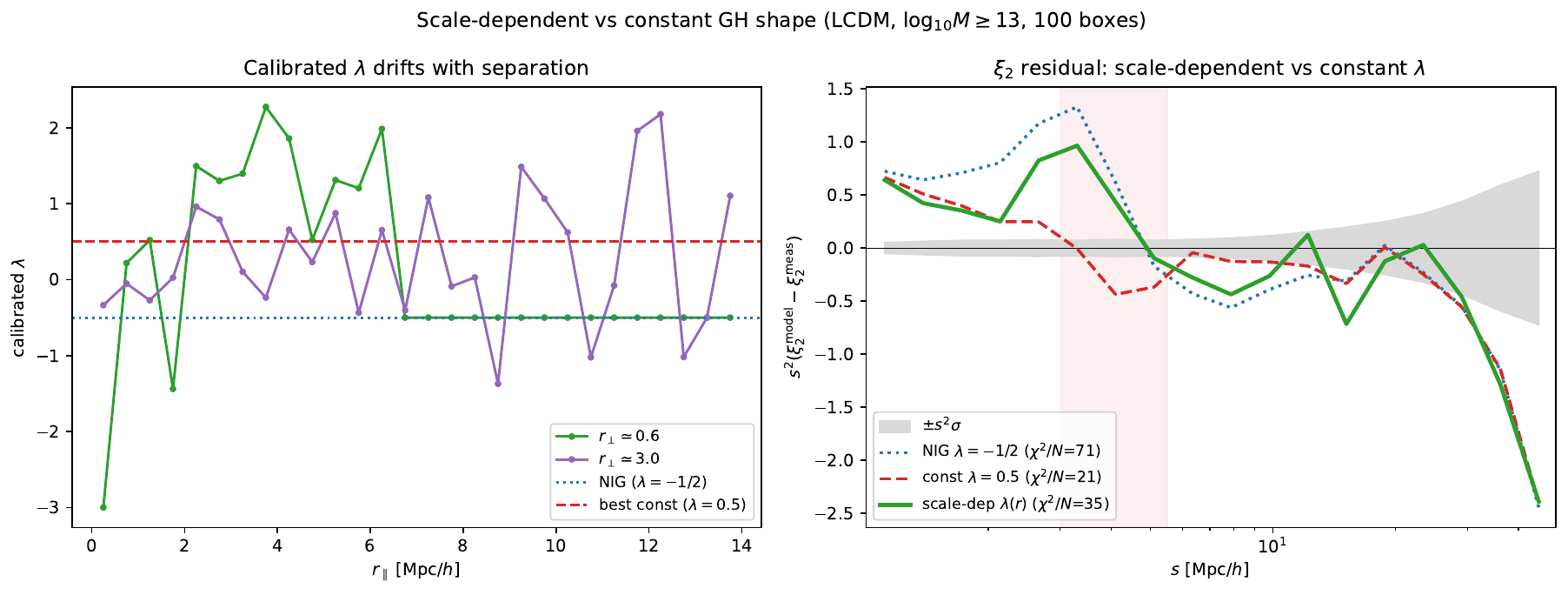
Is a scale-dependent \(\lambda\) worth it?

No. This was tested two independent ways and both agree.

Calibrating on the PDF shape (per-cell KL divergence) actually loses to a well-chosen constant \(\lambda\): the per-cell \(\lambda(r)\) lands at \(\chi^2/\mathrm{ndof}=35\) versus \(21\) for a constant \(\lambda\simeq0.5\), both far below NIG's \(71\).

Calibrating on the \(\xi_2\) observable itself lets a scale-dependent \(\lambda(r)=a+b\ln r\) nudge ahead in-sample (LCDM \(\log_{10}M\ge13\): \(20.7\) vs \(21.7\) full, and a real ~30% gain in the dip). But it does not generalise: refit independently across four masses and on \(f(R)\), the slope \(b\) has no consistent sign, the full-range gains are all \(\lesssim1\) in \(\chi^2/\mathrm{ndof}\), and on the out-of-distribution \(f(R)\) sample \(\lambda(r)\) is worse than the constant — the signature of overfitting.

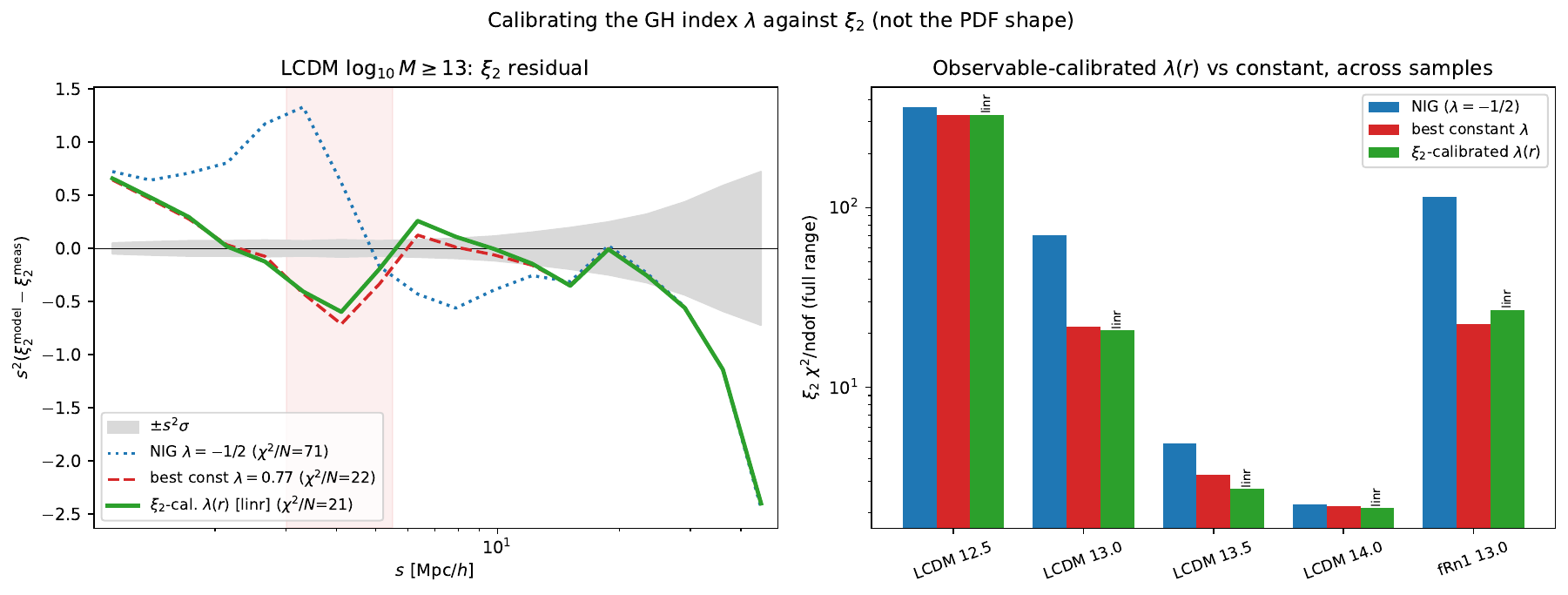
Bottom line

Recommended velocity-PDF ladder

NIG (analytic, zero-tuning) → a single tuned constant-\(\lambda\) GHD → a measured-PDF emulator for the last percent. A scale-dependent \(\lambda(r)\) is not worth the extra parameter.

See Velocity PDFs for the models and the moment→parameter maths.